 StarCraft II Reinforcement Learning
StarCraft II is widely considered one of the most challenging environments for artificial intelligence. Unlike the simple Cartpole environment we tackled, SC2 is a real-time strategy game with an enormous action space, partial observability, and a time scale that makes it difficult to train using traditional reinforcement learning methods. What makes SC2 particularly fascinating is that mastering even its simplest tasks requires an agent to process visual observations at the pixel level and learn complex motor skills — no hand-crafted features allowed. In this project, we'll use deep reinforcement learning to teach an AI agent how to complete one of the most basic StarCraft II training maps: MoveToBeacon.
MoveToBeacon is part of the SMAC (StarCraft Multi-Agent Challenge) suite of maps designed by DeepMind to evaluate reinforcement learning agents in a controlled setting. The objective is deceptively simple: the agent controls a marine and must move it to a glowing beacon that appears somewhere on the map. That's it — no enemies, no resource gathering, just navigate to a target. However, "simple" doesn't mean "easy." The agent receives raw screen and minimap data as input, processes it through a convolutional neural network, and must learn to issue the correct movement commands entirely on its own.
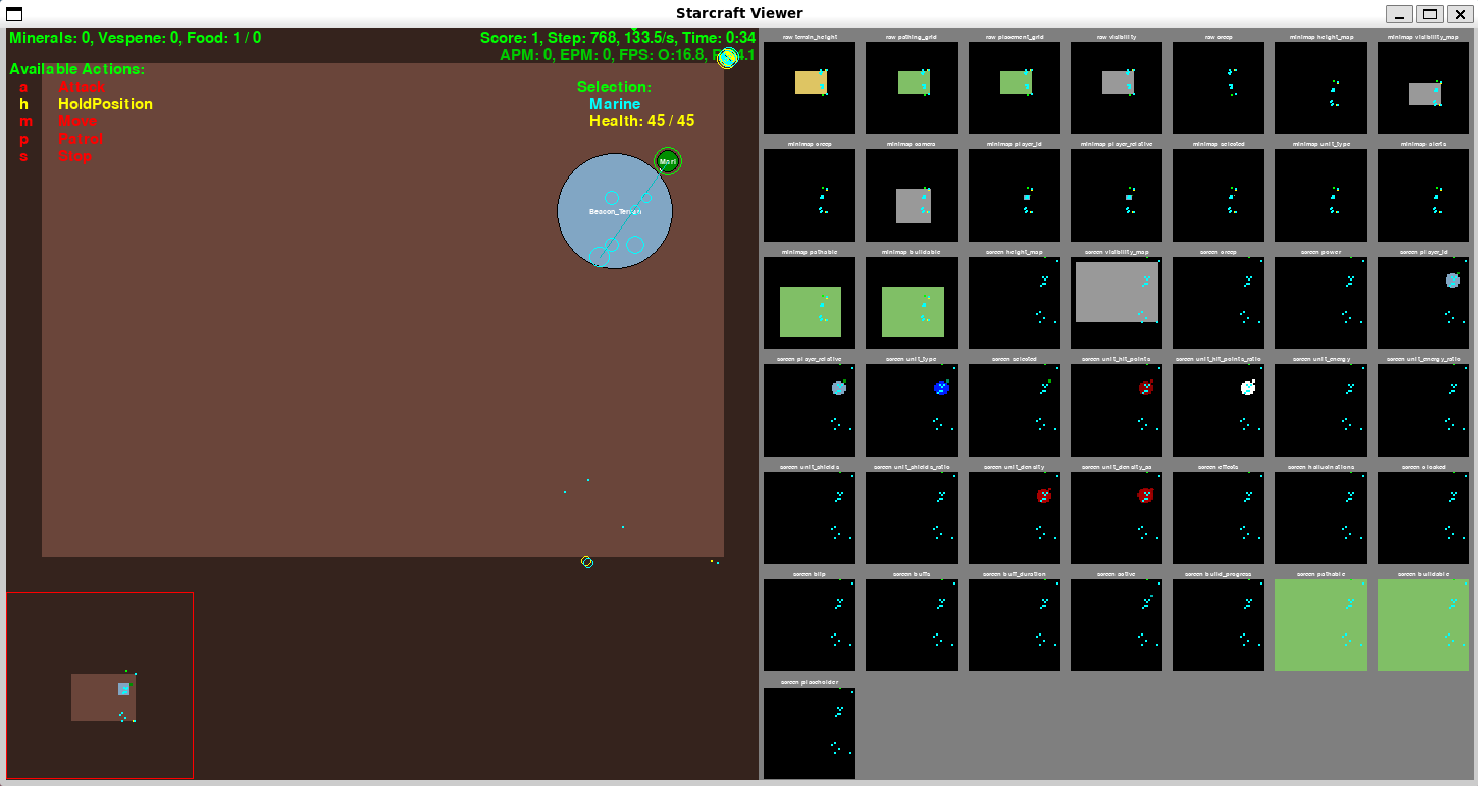
But before our agent can even think about moving units, it first needs to be able to see. The above screenshot shows what the agent perceives at each step — rendered using PyGame for debugging purposes. The agent receives three distinct types of observations through the PySC2 API. The feature_screen layer contains spatial information about units, terrain, and effects in the local viewport. The feature_minimap layer provides an overhead view of the entire map, showing unit positions and fog of war. Finally, the flat features are non-spatial scalar values like mineral count, vespene count, army size, and food capacity — essentially the agent's "HUD." Together, these three modalities give the agent everything it needs to understand its situation, but processing them effectively requires a carefully designed network.
The network architecture is based on the FullyConv model from DeepMind's paper on parameterized action spaces. Rather than flattening the screen and minimap into a giant vector (which would destroy all spatial structure), the network processes each modality through its own convolutional tower before fusing them together.
class FullyConv(nn.Module):
    def __init__(self, data_format='NCHW'):
        super().__init__()
        self.data_format = data_format

        # Screen input conv
        self.screen_conv1 = nn.Conv2d(
            in_channels=screen_embedding_channels(),
            out_channels=16, kernel_size=5, stride=1, padding=2)
        self.screen_conv2 = nn.Conv2d(16, 32, kernel_size=3, stride=1, padding=1)

        # Minimap input conv
        self.minimap_conv1 = nn.Conv2d(
            in_channels=minimap_embedding_channels(),
            out_channels=16, kernel_size=5, stride=1, padding=2)
        self.minimap_conv2 = nn.Conv2d(16, 32, kernel_size=3, stride=1, padding=1)

        # Embedding layers
        self.flat_embed_fc = nn.Linear(sum(feat_embedding_dims(FLAT_FEATURES)), 32)

        # Shared FC layer
        input_features = (32 + 32 + 32) * spatial_output_size()
        self.fc = nn.Linear(input_features, 256)

        # Value head
        self.value_head = nn.Linear(256, 1)

        # Policy heads
        self.fn_head = nn.Linear(256, NUM_FUNCTIONS)
        # ... spatial and non-spatial argument heads ...
Notice how the screen and minimap each get their own pair of convolutional layers — a wider 5x5 filter followed by a narrower 3x3 filter — that gradually compress spatial information into 32-channel feature maps. The flat features are projected to 32 dimensions using a linear layer, then broadcast across the spatial dimensions to match. All three 32-channel maps are concatenated and flattened before passing through a shared fully-connected layer with 256 units. From there, the network splits into two heads: a policy head that outputs action probabilities, and a value head that estimates the expected return from the current state.
One important detail: since many of the screen and minimap features are categorical (not continuous), feeding them directly into convolutions would imply an ordinal relationship that doesn't exist. To handle this, the network uses learnable embedding layers — for each categorical feature with scale S, we create a one-hot encoding and pass it through a 1x1 convolution that produces round(log2(S)) output channels. This dimensionality reduction is crucial: it compresses high-cardinality categorical features (like unit types) into dense, learnable representations without blowing up the number of parameters.
Now for the training algorithm. We're using Advantage Actor-Critic (A2C), a policy gradient method that combines the best of two approaches: a "policy" that directly outputs action probabilities, and a "value function" that estimates how good a given state is. The "advantage" in A2C refers to the difference between the actual return received and the value the network predicted — this advantage signal tells the policy whether a particular action was better or worse than expected.
            # Loss components computed during training:

            # Policy loss: maximize log-prob of taken actions, weighted by advantage
            policy_loss = -torch.mean(advs_normalized * log_probs)

            # Value loss: minimize the difference between predicted and actual returns
            value_loss = torch.mean(torch.square(returns_t - value) / 2.0)

            # Entropy bonus: encourage exploration by maximizing policy entropy
            entropy = _compute_policy_entropy(available_actions, policy, actions)

            # Combined loss
            loss = (policy_loss
                    + value_loss * self.value_loss_weight
                    - entropy * self.entropy_weight)
The policy loss pushes the network to assign higher probability to actions that yielded positive advantages. The value loss trains the value head to produce accurate return estimates, which in turn stabilizes the advantage signal. And the entropy bonus is a subtle but important detail — by encouraging the policy to maintain high entropy, we prevent it from converging too early on suboptimal actions. I've found that getting the balance between these three terms right is more art than science, and a lot of hyperparameter tuning goes into finding the right weights for each.
Training in StarCraft II is notoriously slow because each game step takes time to simulate. To speed things up, we run 32 parallel environments across separate processes using Python\'s multiprocessing module. Each environment runs its own copy of the SC2 game, and at each step, the agent collects observations from all 32 environments simultaneously before performing a single training update. This approach is borrowed from OpenAI Baselines\' SubprocVecEnv, and it makes a massive difference in wall-clock training time.
To run training on MoveToBeacon, you just need to execute the <code>run.py</code> script with an experiment ID:
python run.py my_sc2_experiment --map MoveToBeacon --visThe --vis flag opens a PyGame window that renders the observation layers in real time, which is incredibly useful for debugging — you can actually watch the agent's "vision" as it learns. After enough training iterations, the agent should reliably navigate its marine to the beacon.
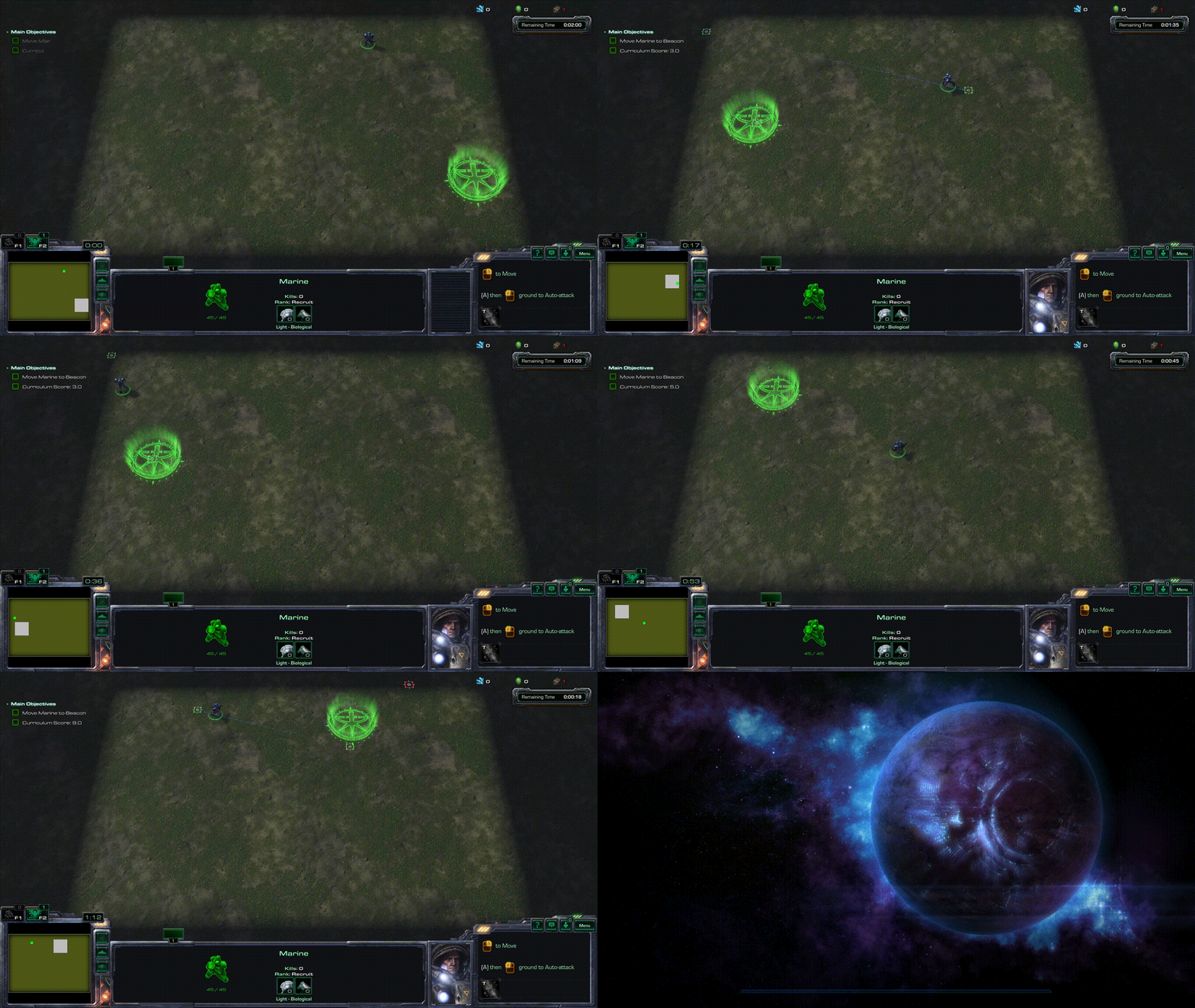
The GIF at the top of this page shows a trained agent completing the MoveToBeacon task. You can see the agent issuing move commands to its marine and guiding it toward the beacon — all learned from scratch using raw observations and no hand-crafted navigation logic. It might not look like much at first glance, but under the hood, this same architecture scales to significantly more complex StarCraft II tasks. The concepts covered here — processing multi-modal observations through convolutional towers, policy gradient optimization with advantage estimation, and parallel environment execution — are all recurring themes in nearly every advanced reinforcement learning system.
If you're curious to learn more, feel free to drop me a line.